As the computing power grows the implementation of Artificial Neural Networks (ANN) becomes more and more common in computational systems and programs. Here it is explained what a simple feedforward artificial neural network is and how it is supposed to work.  This article is a demonstration about the R library neuralnet [1a,b] and how it can be applied.

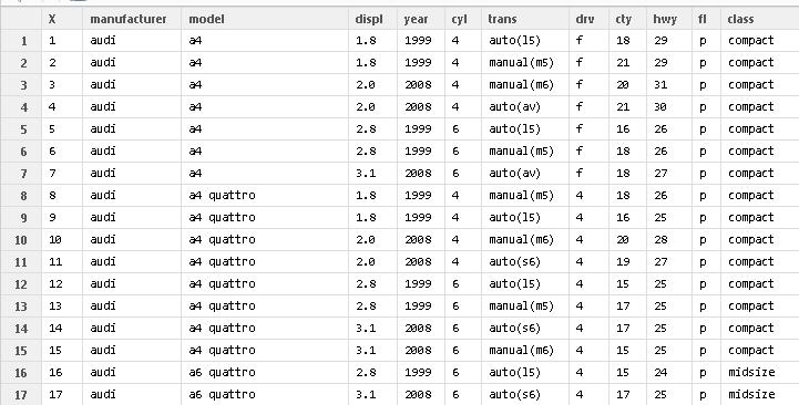
The neuralnet package was applied on a dataset called mpg which shows a list of cars and their gas consumption per mile. There are also many other datasets that can be used for training with data [2].

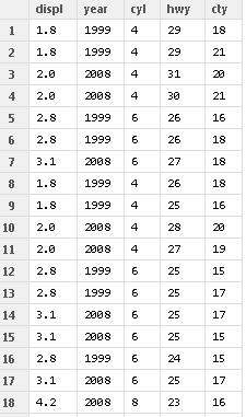
The first step is to look at our data and decide what we need and how should they look in order to use them.  The first lines of the code set the working directory and load the library of the neuralnet:

[sourcecode language=”r”]
setwd(choose.dir())
library(neuralnet)
[/sourcecode]

Next the data is imported

[code language=”r”]
datain1<-read.csv(file.choose(),header=T)
[/code]

it should be like this:

[code language=”r”]data <- datain1[, c( ‘displ’, ‘year’, ‘cyl’, ‘hwy’,’cty’)][/code]

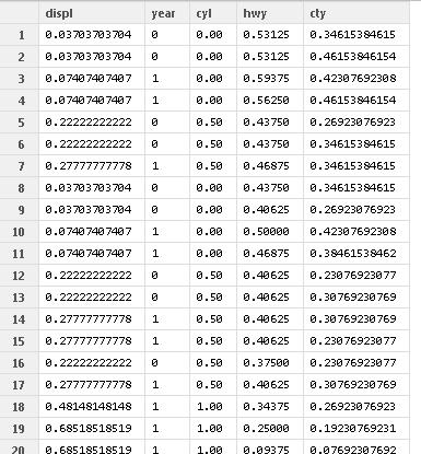
After this we must normalize our data. Database normalization is the process of organizing the fields and tables of a relational database to minimize redundancy and dependency [3]. Bellow it is shown why data should be normalized. Normalization is done with this code:

[code language=”r”]norm.fun = function(x){(x – min(x))/(max(x) – min(x))}data.norm = apply(data, 2, norm.fun)[/code]

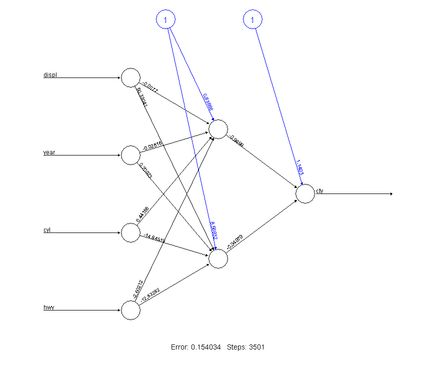
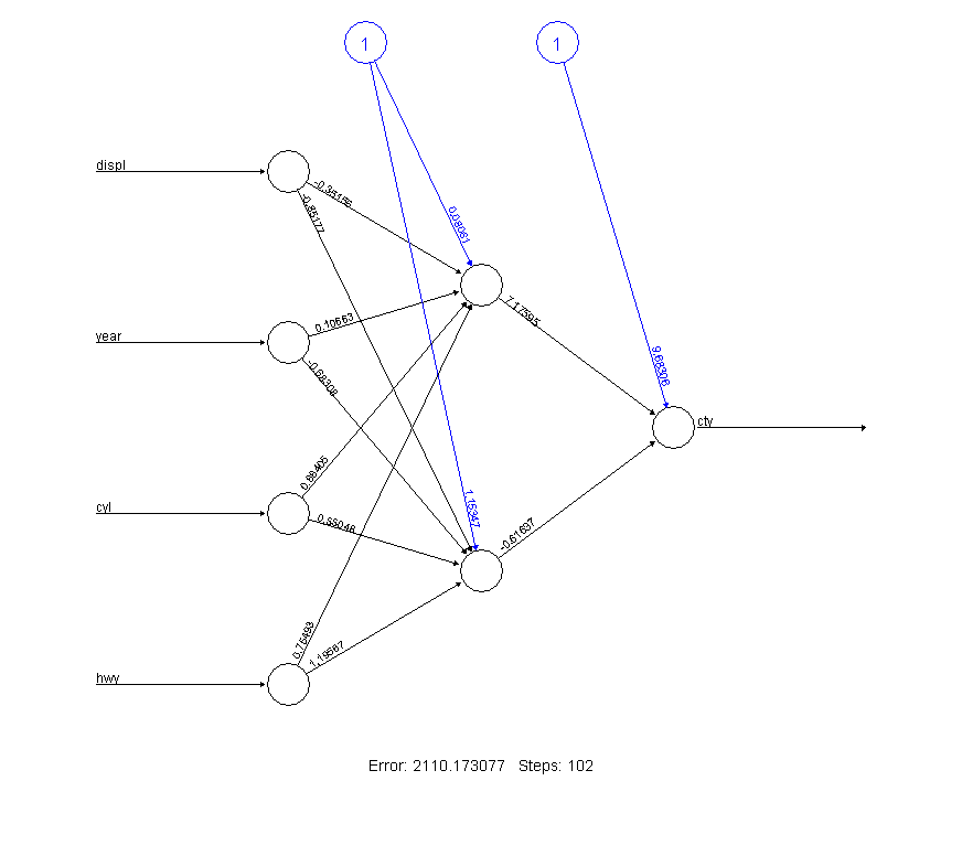
Then we train the ANN that contains 2 hidden layers. We ask for the network to compute the gas consumption in the city while we provide it the other data. The code is:

[code language=”r”]net <- neuralnet(cty ~ displ + year + cyl + hwy, data.norm, hidden = 2)[/code]

We can print the net and see the ERROR [4] we have:

[code language=”r”]print(net)[/code]

and then we can plot our ANN with plot(net) 

*If the data wasn’t normalized we would have a bigger error that would make our ANN inaccurate.

Now it is time to test the Artificial Neural Network and see if it can predict the data we want. A test database is provided.

[code language=”r”]testdata<-read.csv(file.choose(),header=F)[/code]

It is important that we should normalize the test data too, otherwise the data will not be compatible.

[code language=”r”]testdata.norm<-data.frame((testdata[,1] – min(data[, ‘displ’]))/(max(data[, ‘displ’])-min(data[, ‘displ’])),(testdata[,2] – min(data[, ‘year’]))/(max(data[, ‘year’])-min(data[, ‘year’])),(testdata[,3] – min(data[, ‘cyl’]))/(max(data[, ‘cyl’])-min(data[, ‘cyl’])),(testdata[,4] – min(data[, ‘hwy’]))/(max(data[, ‘hwy’])-min(data[, ‘hwy’])))[/code]

We run the network in order to compute the test data output we want.

[code language=”r”]
net.test<-compute(net,testdata.norm)

testouputdata<-net.test$net.result
[/code]

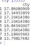
And finally we print the results out denormalized:

[code language=”r”]
print(data.frame(‘cty’=(min(data[, ‘cty’]) + testouputdata * (max(data[, ‘cty’])-min(data[, ‘cty’])))))
[/code]

this is the code for denormalization:

[code language=”r”](min(data[, ‘cty’]) + testouputdata * (max(data[, ‘cty’])-min(data[, ‘cty’])))[/code]

As it can be seen, the data is really close to the real ones!!

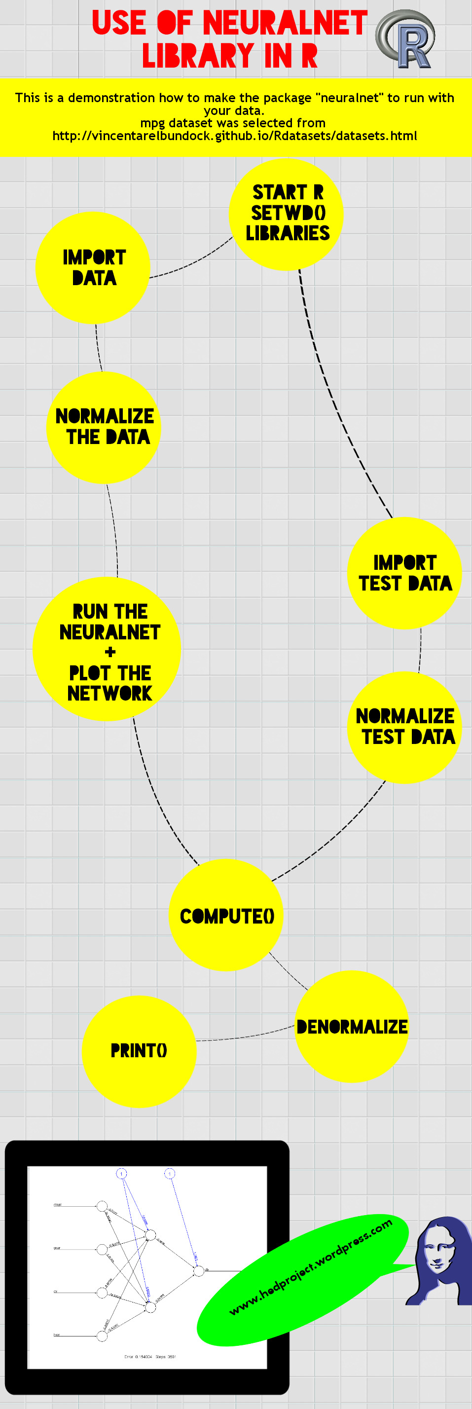
I also made this infogram!!! 😉

References:

1a Frauke Günther and Stefan Fritsch, neuralnet:Training of Neural Networks, R Journal, January 2010.

1b http://cran.r-project.org/web/packages/neuralnet/neuralnet.pdf

2 http://vincentarelbundock.github.io/Rdatasets/datasets.html

3 normalization, http://en.wikipedia.org/wiki/Database_normalization

4 error, http://en.wikipedia.org/wiki/Backpropagation#Intuition