VLOOKUP is probably one of the mostly used Excel functions. It is used when the user needs to find things in a table or a range by row. For example, look up a price of an automotive part by the part number, or find an employee name based on their employee ID.

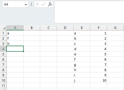
Its usage is quite simple: =VLOOKUP(lookup_value, table_array, column_index_number, [range_lookup]).

• lookup_value is the value you are looking for in the table.
• table_array is the range of cells that contains the table you are searching.
• column_index_number is the column number of the value you want to return. The first column is 1, the second column is 2, and so on.
• range_lookup is a Boolean value that tells Excel whether to do an exact match (TRUE) or an approximate match (FALSE). If you omit this argument, Excel will do an approximate match by default.

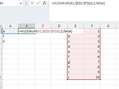
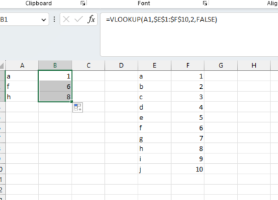
Despite being one of the most used formulas in excel it is not wise to use it in big excel sheets that are required to produce prices, forecasts or do other serious calculations.

The reason is simple. Referring a column without any other references leads to probles as we will see below.

At the picture exaples let’s assume that we want to add a column next to column E and expand our table.

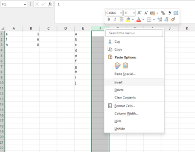
What happens is that the reference still remains the 2nd column of the table which is now zero or might have other values that we would insert.

The previous VLOOKUP formula matching will give us the below:

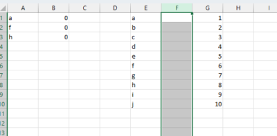
That’s why it is recomended to use a more advanced combination like INDEX MATCH MATCH that it’s reference is tied to the header of the table and not by the column distance from the 1st column of the table we want to match.

To find how INDEX MATCH MATCH works, alongside with other super userful excel formulas visit this page. It’s an absolute MUST KNOW!